Model Results

Import Requisite Libraries

######################## Standard Library Imports ##############################
import pandas as pd
import os
import sys

# Add the parent directory to sys.path to access 'functions.py'
sys.path.append(os.path.join(os.pardir))
from eda_toolkit import ensure_directory

######################## Modeling Library Imports ##############################
import shap
import model_tuner
from model_tuner.pickleObjects import loadObjects
import eda_toolkit
import matplotlib.pyplot as plt

from core.functions import evaluate_kfold_oof, build_multimodel_performance_table, load_model_from_mlflow


# Add the parent directory to sys.path to access 'functions.py'
sys.path.append(os.path.join(os.pardir))

print(
    f"This project uses: \n \n Python {sys.version.split()[0]} \n model_tuner "
    f"{model_tuner.__version__} \n eda_toolkit {eda_toolkit.__version__}"
)

/home/lshpaner/Python_Projects/circ_milan/venv_circ_311/lib/python3.11/site-packages/tqdm/auto.py:21: TqdmWarning: IProgress not found. Please update jupyter and ipywidgets. See https://ipywidgets.readthedocs.io/en/stable/user_install.html
  from .autonotebook import tqdm as notebook_tqdm

This project uses: 
 
 Python 3.11.0 
 model_tuner 0.0.34b1 
 eda_toolkit 0.0.19

Set Paths & Read in the Data

# Define base paths
# `base_path`` represents the parent directory of current working directory
base_path = os.path.join(os.pardir)
# Go up one level from 'notebooks' to the parent directory, then into the 'data' folder

data_path = os.path.join(os.pardir, "data")
image_path_png = os.path.join(base_path, "images", "png_images", "modeling")
image_path_svg = os.path.join(base_path, "images", "svg_images", "modeling")

# Use the function to ensure the 'data' directory exists
ensure_directory(data_path)
ensure_directory(image_path_png)
ensure_directory(image_path_svg)

Directory exists: ../data
Directory exists: ../images/png_images/modeling
Directory exists: ../images/svg_images/modeling

data_path = "../data/processed/"
model_path = "../mlruns/models/"

df = pd.read_parquet(os.path.join(data_path, "X.parquet"))

print(f"DataFrame Columns w/ Outcome:\n{df.columns.to_list()}")
print(f"DataFrame Shape: {df.shape}")

DataFrame Columns w/ Outcome:
['Age_years', 'BMI', 'Surgical_Technique', 'Intraoperative_Blood_Loss_ml', 'Intraop_Mean_Heart_Rate_bpm', 'Intraop_Mean_Pulse_Ox_Percent', 'Surgical_Time_min', 'BMI_Category_Obese', 'BMI_Category_Overweight', 'BMI_Category_Underweight', 'Intraop_SBP', 'Intraop_DBP', 'Diabetes']
DataFrame Shape: (194, 13)

X = pd.read_parquet(os.path.join(data_path, "X.parquet"))
y = pd.read_parquet(os.path.join(data_path, "y_Bleeding_Edema_Outcome.parquet"))
df = df.join(y, how="inner", on="patient_id")

Load Models

# flavor (run name in MLflow) -> algo prefix used in the artifact folder
FLAVORS = {
    "lr_smote_training": "lr",
    "rf_smote_training":  "rf",
    "svm_orig_training": "svm",
}

# ----------------------------------------------------------------------
# load all models
# ----------------------------------------------------------------------
models = {
    flavor: load_model_from_mlflow(flavor, algo)
    for flavor, algo in FLAVORS.items()
}

# keep the original short names working for downstream code
model_lr  = models["lr_smote_training"]
model_rf  = models["rf_smote_training"]
model_svm = models["svm_orig_training"]

Object loaded!
Object loaded!
Object loaded!

Set-up Pipelines, Model Titles, and Thresholds

pipelines_or_models = [model_lr, model_rf, model_svm]

# Model titles
model_titles = [
    "Logistic Regression",
    "Random Forest Classifier",
    "Support Vector Machine",
]


thresholds = {
    "Logistic Regression": next(iter(model_lr.threshold.values())),
    "Random Forest Classifier": next(iter(model_rf.threshold.values())),
    "Support Vector Machine": next(iter(model_svm.threshold.values())),
}

for col in X.columns:
    if col.startswith("BMI_"):
        print(f"Value Counts for column {col}:\n")
        print(X[col].value_counts())
        print("\n")

Value Counts for column BMI_Category_Obese:

BMI_Category_Obese
0    183
1     11
Name: count, dtype: int64


Value Counts for column BMI_Category_Overweight:

BMI_Category_Overweight
0    141
1     53
Name: count, dtype: int64


Value Counts for column BMI_Category_Underweight:

BMI_Category_Underweight
0    190
1      4
Name: count, dtype: int64

Summarize Model Performance

from model_metrics import summarize_model_performance

table3 = summarize_model_performance(
    model=pipelines_or_models,
    X=X,
    y=y,
    model_title=model_titles,
    model_threshold=thresholds,
    return_df=True,
)

Running k-fold model metrics...

Processing Folds: 100%|██████████| 10/10 [00:00<00:00, 10.33it/s]

Running k-fold model metrics...

Processing Folds: 100%|██████████| 10/10 [00:01<00:00,  9.52it/s]

Running k-fold model metrics...

Processing Folds: 100%|██████████| 10/10 [00:00<00:00, 126.79it/s]

table3

	Metrics	Logistic Regression	Random Forest Classifier	Support Vector Machine
	Precision/PPV	0.571	0.706	0.725
	Average Precision	0.809	0.737	0.832
	Sensitivity/Recall	0.897	0.828	0.862
	Specificity	0.713	0.853	0.860
	F1-Score	0.698	0.762	0.787
	AUC ROC	0.900	0.887	0.907
	Brier Score	0.137	0.105	0.105
	Model Threshold	0.439	0.318	0.238

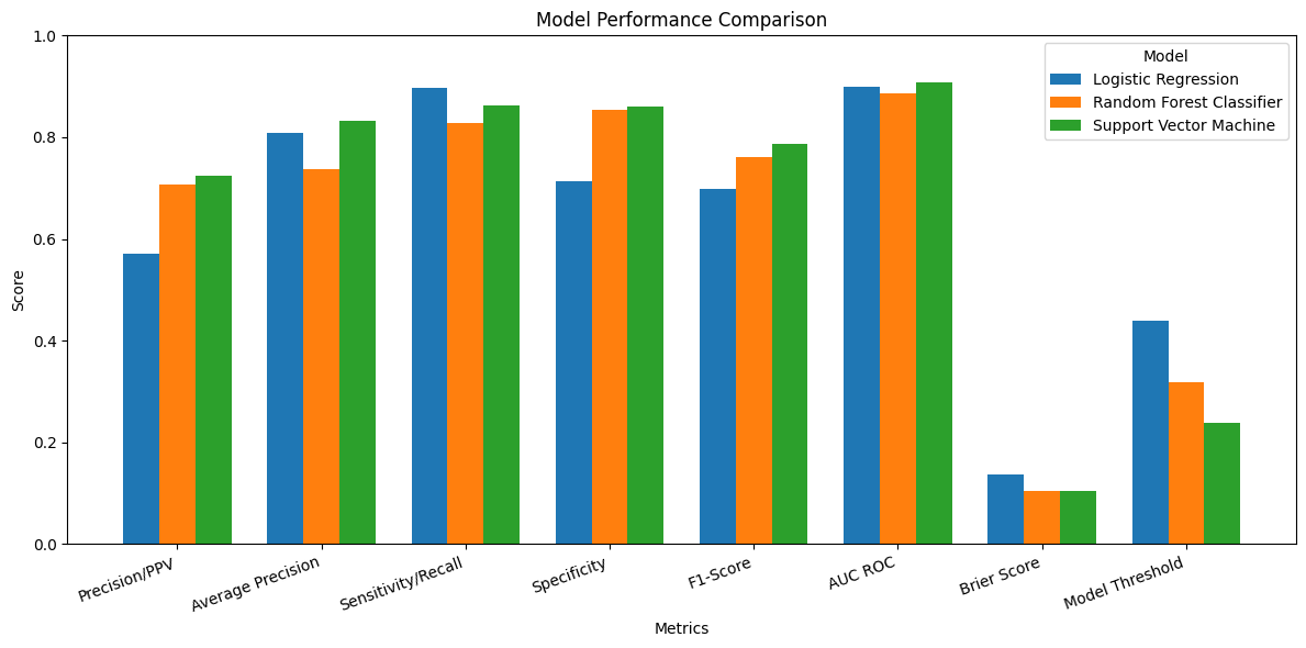
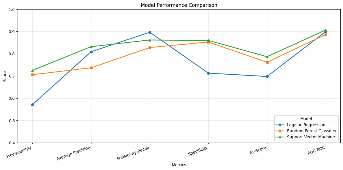
import numpy as np
import matplotlib.pyplot as plt

df_bar = table3.set_index('Metrics')   # if 'Metrics' is already the index, drop this line

x = np.arange(len(df_bar.index))
width = 0.25

fig, ax = plt.subplots(figsize=(12, 6))
for i, model in enumerate(df_bar.columns):
    ax.bar(x + (i - 1) * width, df_bar[model], width, label=model)

ax.set_xlabel('Metrics')
ax.set_ylabel('Score')
ax.set_title('Model Performance Comparison')
ax.set_xticks(x)
ax.set_xticklabels(df_bar.index, rotation=20, ha='right')
ax.set_ylim(0, 1.0)
ax.legend(title='Model', loc='upper right')
plt.tight_layout()
plt.savefig(os.path.join(image_path_png, "model_performance_comparison.png"), dpi=300)
plt.savefig(os.path.join(image_path_svg, "model_performance_comparison.svg"))
plt.show()

import matplotlib.pyplot as plt

keep = ['Precision/PPV', 'Average Precision', 'Sensitivity/Recall',
        'Specificity', 'F1-Score', 'AUC ROC']

df_line = table3[table3['Metrics'].isin(keep)].set_index('Metrics').loc[keep]

fig, ax = plt.subplots(figsize=(12, 6))
markers = {'Logistic Regression': 'o', 'Random Forest Classifier': 's',
           'Support Vector Machine': '^'}

for model in df_line.columns:
    ax.plot(df_line.index, df_line[model], marker=markers.get(model, 'o'),
            linewidth=2, label=model)

ax.set_xlabel('Metrics')
ax.set_ylabel('Score')
ax.set_title('Model Performance Comparison')
ax.set_ylim(0.4, 1.0)
ax.grid(True, alpha=0.3)
ax.legend(title='Model', loc='lower right')
plt.xticks(rotation=20, ha='right')
plt.tight_layout()
plt.savefig(os.path.join(image_path_png, "model_performance_comparison_line.png"), dpi=300)
plt.savefig(os.path.join(image_path_svg, "model_performance_comparison_line.svg"))
plt.show()

Bootstrapped Model Performance Comparison

We first generate pooled out-of-fold (OOF) predictions using stratified K-fold cross-validation, ensuring that each observation is evaluated by a model that did not see it during training. These OOF predictions provide an unbiased estimate of generalization performance.

We then compute point estimates for each metric on the pooled OOF predictions and estimate 95% confidence intervals using a nonparametric bootstrap. Each bootstrap resample draws n observations with replacement from the OOF dataset, and metrics are recomputed on each resample. This separates model fitting (handled by CV) from uncertainty estimation (handled by bootstrapping), avoiding optimistic bias.

model_lr_kfold_oof = evaluate_kfold_oof(
    model=model_lr,
    X=X,
    y=y,
    n_splits=10,
    threshold=thresholds["Logistic Regression"],
    random_state=222,
)
model_rf_kfold_oof = evaluate_kfold_oof(
    model=model_rf,
    X=X,
    y=y,
    n_splits=10,
    threshold=thresholds["Random Forest Classifier"],
    random_state=222,
)
model_svm_kfold_oof = evaluate_kfold_oof(
    model=model_svm,
    X=X,
    y=y,
    n_splits=10,
    threshold=thresholds["Support Vector Machine"],
    random_state=222,
)

# Evaluate k-fold OOF predictions
y_true_oof_lr = model_lr_kfold_oof["y_true_oof"]  # eval for lr
y_prob_oof_lr = model_lr_kfold_oof["y_prob_oof"]

y_true_oof_rf = model_rf_kfold_oof["y_true_oof"]  # eval for rf
y_prob_oof_rf = model_rf_kfold_oof["y_prob_oof"]

y_true_oof_svm = model_svm_kfold_oof["y_true_oof"]  # eval for svm
y_prob_oof_svm = model_svm_kfold_oof["y_prob_oof"]

boots_metrics = [
    "precision",
    "average_precision",
    "recall",
    "specificity",
    "f1_weighted",
    "roc_auc",
    "brier_score",
]

METRICS = [
    "precision",
    "average_precision",
    "recall",
    "specificity",
    "f1_weighted",
    "roc_auc",
    "brier_score",
]

# Extract shared ground truth ONCE
y_true_oof = model_lr_kfold_oof["y_true_oof"]


# Build table
performance_table = build_multimodel_performance_table(
    y_true_oof=y_true_oof,
    models_dict={
        "Logistic Regression": {
            "y_prob": model_lr_kfold_oof["y_prob_oof"],
            "y_pred": model_lr_kfold_oof["y_pred_oof"],
        },
        "Random Forest": {
            "y_prob": model_rf_kfold_oof["y_prob_oof"],
            "y_pred": model_rf_kfold_oof["y_pred_oof"],
        },
        "SVM": {
            "y_prob": model_svm_kfold_oof["y_prob_oof"],
            "y_pred": model_svm_kfold_oof["y_pred_oof"],
        },
    },
    metrics=METRICS,
    n_bootstrap=1000,
)

Bootstrapping metrics: 100%|██████████| 21000/21000 [00:10<00:00, 1954.81resample/s]

performance_table

	Model	Metric	Point Estimate	95% CI
0	Logistic Regression	Precision	0.571	0.469–0.663
1	Logistic Regression	Average Precision	0.809	0.704–0.899
2	Logistic Regression	Recall	0.897	0.817–0.966
3	Logistic Regression	Specificity	0.713	0.632–0.783
4	Logistic Regression	F1 Weighted	0.698	0.603–0.778
5	Logistic Regression	Roc Auc	0.900	0.849–0.943
6	Logistic Regression	Brier Score	0.137	0.117–0.160
7	Random Forest	Precision	0.706	0.596–0.810
8	Random Forest	Average Precision	0.737	0.613–0.875
9	Random Forest	Recall	0.828	0.719–0.917
10	Random Forest	Specificity	0.853	0.786–0.910
11	Random Forest	F1 Weighted	0.762	0.667–0.837
12	Random Forest	Roc Auc	0.887	0.826–0.940
13	Random Forest	Brier Score	0.105	0.077–0.136
14	SVM	Precision	0.725	0.623–0.826
15	SVM	Average Precision	0.832	0.735–0.913
16	SVM	Recall	0.862	0.765–0.939
17	SVM	Specificity	0.860	0.797–0.915
18	SVM	F1 Weighted	0.787	0.706–0.857
19	SVM	Roc Auc	0.907	0.855–0.950
20	SVM	Brier Score	0.105	0.077–0.134

SHAP Summary Plot

SHAP (SHapley Additive exPlanations) Set-up

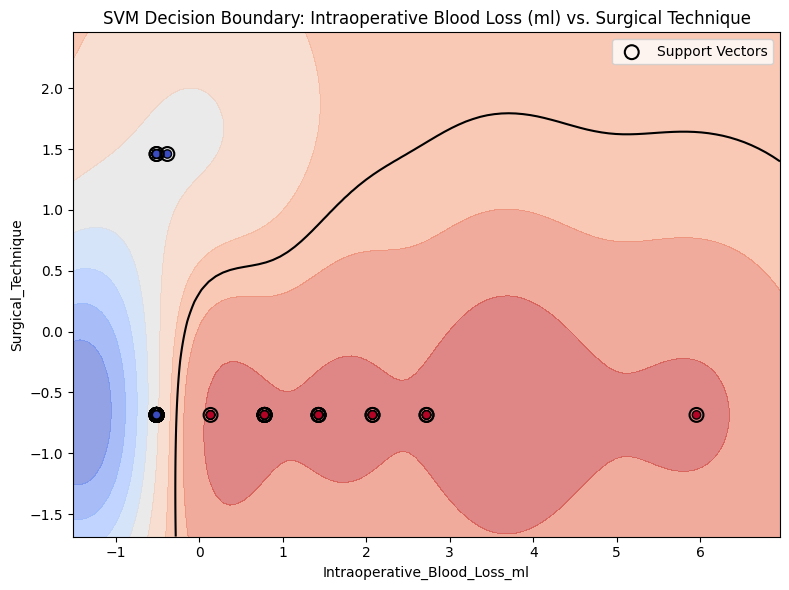
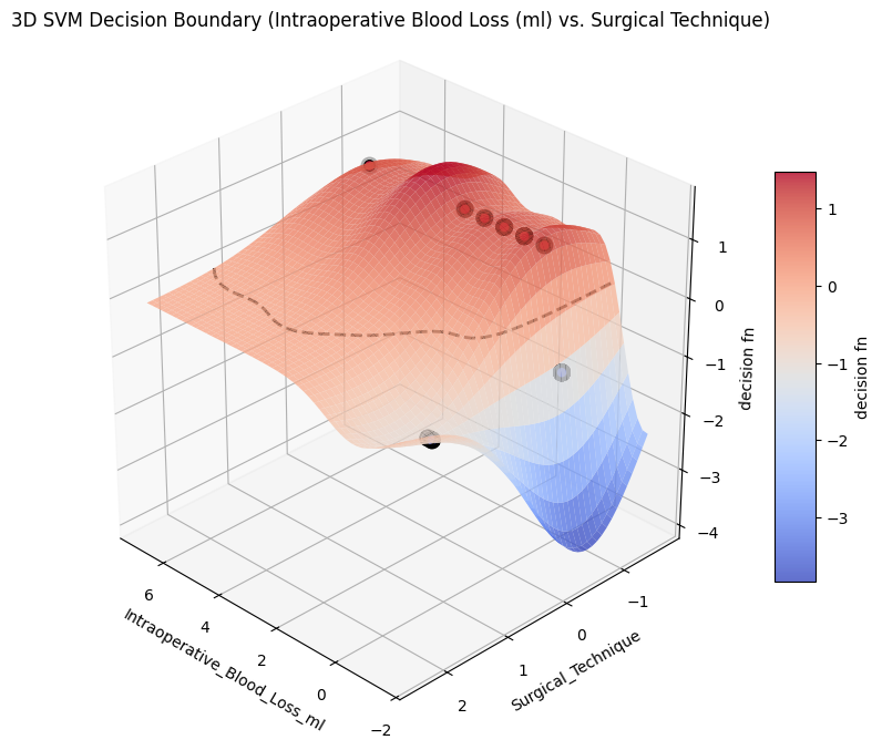
# Step 1: Get transformed features using model's preprocessing pipeline
X_transformed = model_svm.get_preprocessing_and_feature_selection_pipeline().transform(
    X
)

# Optional: Sampling for speed (or just use X_transformed if it's small)
sample_size = 100
X_sample = shap.utils.sample(X_transformed, sample_size, random_state=42)

# Step 2: Get final fitted model (SVC in pipeline)
final_model = model_svm.estimator.named_steps[model_svm.estimator_name]


# Step 3: Define a pred. function that returns only the probability for class 1
def model_predict(X):
    return final_model.predict_proba(X)[:, 1]


# Step 4: Create SHAP explainer
explainer = shap.KernelExplainer(
    model_predict, X_sample, feature_names=model_svm.get_feature_names()
)

# Step 5: Compute SHAP values for the full dataset or sample
shap_values = explainer.shap_values(X_sample)  # can use X_transformed instead

100%|██████████| 100/100 [00:58<00:00,  1.71it/s]

SHAP Beeswarm Plot

# Step 6a: SHAP beeswarm plot (default)
shap.summary_plot(
    shap_values,
    X_sample,
    feature_names=model_svm.get_feature_names(),
    show=False,
)

plt.savefig(os.path.join(image_path_png, "shap_summary_beeswarm.png"), dpi=600)
plt.savefig(os.path.join(image_path_svg, "shap_summary_beeswarm.svg"), dpi=600)

SHAP Bar Plot

# Step 6b: SHAP bar plot (mean |SHAP value| for each feature)
shap.summary_plot(
    shap_values,
    X_sample,
    feature_names=model_svm.get_feature_names(),
    plot_type="bar",
    show=False,
)

plt.savefig(os.path.join(image_path_png, "shap_summary_bar.png"), dpi=600)
plt.savefig(os.path.join(image_path_svg, "shap_summary_bar.svg"), dpi=600)

Plot SVM Decision Boundary

from project_functions import plot_svm_decision_boundary_2d

plot_svm_decision_boundary_2d(
    # model=model_svm,
    X=X,
    y=y,
    feature_pair=("Intraoperative_Blood_Loss_ml", "Surgical_Technique"),
    title="SVM Decision Boundary: Intraoperative Blood Loss (ml) vs. Surgical Technique",
    image_path_svg=os.path.join(image_path_svg, "svm_decision_surface_2d.svg"),
)

from project_functions import plot_svm_decision_boundary_2d

plot_svm_decision_boundary_2d(
    # model=model_svm,
    X=X,
    y=y,
    feature_pair=("Intraoperative_Blood_Loss_ml", "Surgical_Technique"),
    title="SVM Decision Boundary: Intraoperative Blood Loss (ml) vs. Surgical Technique",
    margin=True,
    image_path_svg=os.path.join(image_path_svg, "svm_decision_surface_2d_margin.svg"),
)

from project_functions import plot_svm_decision_surface_3d

plot_svm_decision_surface_3d(
    X=X,
    y=y,
    # figsize=(6, 10),
    feature_pair=("Intraoperative_Blood_Loss_ml", "Surgical_Technique"),
    title="3D SVM Decision Boundary (Intraoperative Blood Loss (ml) vs. Surgical Technique)",
    image_path_png=os.path.join(image_path_png, "svm_decision_surface_3d.png"),
    image_path_svg=os.path.join(image_path_svg, "svm_decision_surface_3d.svg"),
)

from project_functions import plot_svm_decision_surface_3d_plotly

# Plotly 3D SVM Decision Surface
plot_svm_decision_surface_3d_plotly(
    X=df,
    y=df["Bleeding_Edema_Outcome"],
    feature_pair=("Intraoperative_Blood_Loss_ml", "Surgical_Technique"),
    title=f"Interactive 3D SVM Decision Boundary:<br>Intraoperative Blood "
    f"Loss (ml) vs. Surgical Technique",
    html_path=os.path.join(image_path_svg, "svm_decision_surface_3d_plotly.html"),
)

Saved interactive plot to ../images/svg_images/modeling/svm_decision_surface_3d_plotly.html

Calibration

# Plot calibration curves in overlay mode
from model_metrics import show_calibration_curve

show_calibration_curve(
    model=pipelines_or_models[0:3],
    X=X,
    y=y,
    model_title=model_titles[0:3],
    overlay=True,
    title="",
    save_plot=True,
    image_path_png=image_path_png,
    image_path_svg=image_path_svg,
    text_wrap=40,
    curve_kwgs={
        "Logistic Regression": {"color": "blue", "linewidth": 1},
        "Support Vector Machine": {
            "color": "red",
            # "linestyle": "--",
            "linewidth": 1.5,
        },
        "Random Forest": {
            "color": "lightblue",
            "linestyle": "--",
            "linewidth": 1.5,
        },
    },
    figsize=(12, 6),
    label_fontsize=10,
    tick_fontsize=10,
    bins=10,
    show_brier_score=True,
    brier_decimals=3,
    subplots=False,
    # gridlines=False,
    linestyle_kwgs={"color": "black"},
)

Running k-fold model metrics...

Processing Folds: 100%|██████████| 10/10 [00:00<00:00, 45.90it/s]

Running k-fold model metrics...

Processing Folds: 100%|██████████| 10/10 [00:01<00:00,  9.94it/s]

Running k-fold model metrics...

Processing Folds: 100%|██████████| 10/10 [00:00<00:00, 127.90it/s]

Confusion Matrices

from model_metrics import show_confusion_matrix

show_confusion_matrix(
    model=pipelines_or_models,
    X=X,
    y=y,
    model_title=model_titles,
    model_threshold=[thresholds],
    # class_labels=["No Pain", "Class 1"],
    cmap="Blues",
    text_wrap=40,
    save_plot=True,
    image_path_png=image_path_png,
    image_path_svg=image_path_svg,
    grid=True,
    n_cols=3,
    n_rows=1,
    figsize=(4, 4),
    show_colorbar=False,
    subplots=True,
    label_fontsize=14,
    tick_fontsize=12,
    inner_fontsize=12,
    class_report=True,
    # thresholds=thresholds,
    # custom_threshold=0.5,
    # labels=False,
)

Running k-fold model metrics...

Processing Folds: 100%|██████████| 10/10 [00:00<00:00, 26.74it/s]

Confusion Matrix for Logistic Regression: 

          Predicted 0  Predicted 1
Actual 0           97           39
Actual 1            6           52

Classification Report for Logistic Regression: 

              precision    recall  f1-score   support

           0       0.94      0.71      0.81       136
           1       0.57      0.90      0.70        58

    accuracy                           0.77       194
   macro avg       0.76      0.80      0.75       194
weighted avg       0.83      0.77      0.78       194


Running k-fold model metrics...

Processing Folds: 100%|██████████| 10/10 [00:01<00:00, 10.00it/s]

Confusion Matrix for Random Forest Classifier: 

          Predicted 0  Predicted 1
Actual 0          116           20
Actual 1           10           48

Classification Report for Random Forest Classifier: 

              precision    recall  f1-score   support

           0       0.92      0.85      0.89       136
           1       0.71      0.83      0.76        58

    accuracy                           0.85       194
   macro avg       0.81      0.84      0.82       194
weighted avg       0.86      0.85      0.85       194


Running k-fold model metrics...

Processing Folds: 100%|██████████| 10/10 [00:00<00:00, 131.63it/s]

Confusion Matrix for Support Vector Machine: 

          Predicted 0  Predicted 1
Actual 0          117           19
Actual 1            8           50

Classification Report for Support Vector Machine: 

              precision    recall  f1-score   support

           0       0.94      0.86      0.90       136
           1       0.72      0.86      0.79        58

    accuracy                           0.86       194
   macro avg       0.83      0.86      0.84       194
weighted avg       0.87      0.86      0.86       194

ROC AUC Curves

from model_metrics import show_roc_curve

# Plot ROC curves
show_roc_curve(
    model=pipelines_or_models,
    X=X,
    y=y,
    overlay=False,
    model_title=model_titles,
    decimal_places=3,
    # n_cols=3,
    # n_rows=1,
    # curve_kwgs={
    #     "Logistic Regression": {"color": "blue", "linewidth": 2},
    #     "SVM": {"color": "red", "linestyle": "--", "linewidth": 1.5},
    # },
    # linestyle_kwgs={"color": "grey", "linestyle": "--"},
    save_plot=True,
    subplots=True,
    n_cols=3,
    figsize=(12, 4),
    # label_fontsize=16,
    # tick_fontsize=16,
    image_path_png=image_path_png,
    image_path_svg=image_path_svg,
    # gridlines=False,
)

Running k-fold model metrics...

Processing Folds: 100%|██████████| 10/10 [00:00<00:00, 56.14it/s]

AUC for Logistic Regression: 0.900

Running k-fold model metrics...

Processing Folds: 100%|██████████| 10/10 [00:01<00:00,  9.61it/s]

AUC for Random Forest Classifier: 0.887

Running k-fold model metrics...

Processing Folds: 100%|██████████| 10/10 [00:00<00:00, 131.47it/s]

AUC for Support Vector Machine: 0.907

show_roc_curve(
    model=pipelines_or_models,
    X=X,
    y=y,
    overlay=True,
    model_title=model_titles,
    title="AUC ROC - All Models",
    curve_kwgs={
        "Logistic Regression": {"color": "blue", "linewidth": 1},
        "Random Forest": {"color": "lightblue", "linewidth": 1},
        "Support Vector Machine": {
            "color": "red",
            "linestyle": "-",
            "linewidth": 2,
        },
    },
    linestyle_kwgs={"color": "grey", "linestyle": "--"},
    save_plot=True,
    subplots=False,
    decimal_places=3,
    figsize=(8, 6),
    # gridlines=False,
    label_fontsize=16,
    tick_fontsize=13,
    image_path_png=image_path_png,
    image_path_svg=image_path_svg,
)

Running k-fold model metrics...

Processing Folds: 100%|██████████| 10/10 [00:00<00:00, 57.24it/s]

AUC for Logistic Regression: 0.900

Running k-fold model metrics...

Processing Folds: 100%|██████████| 10/10 [00:01<00:00,  9.77it/s]

AUC for Random Forest Classifier: 0.887

Running k-fold model metrics...

Processing Folds: 100%|██████████| 10/10 [00:00<00:00, 137.29it/s]

AUC for Support Vector Machine: 0.907

Precision-Recall Curves

from model_metrics import show_pr_curve

# Plot PR curves
show_pr_curve(
    model=pipelines_or_models,
    X=X,
    y=y,
    # x_label="Hello",
    model_title=model_titles,
    decimal_places=3,
    overlay=False,
    subplots=True,
    save_plot=True,
    image_path_png=image_path_png,
    image_path_svg=image_path_svg,
    figsize=(12, 4),
    n_cols=3,
    # tick_fontsize=16,
    # label_fontsize=16,
    # grid=True,
    # gridlines=False,
)

Running k-fold model metrics...

Processing Folds: 100%|██████████| 10/10 [00:00<00:00, 56.27it/s]

Average Precision for Logistic Regression: 0.809

Running k-fold model metrics...

Processing Folds: 100%|██████████| 10/10 [00:01<00:00,  9.94it/s]

Average Precision for Random Forest Classifier: 0.737

Running k-fold model metrics...

Processing Folds: 100%|██████████| 10/10 [00:00<00:00, 133.69it/s]

Average Precision for Support Vector Machine: 0.832

show_pr_curve(
    model=pipelines_or_models,
    X=X,
    y=y,
    overlay=True,
    model_title=model_titles[0:3],
    title="Precision-Recall - All Models",
    curve_kwgs={
        "Logistic Regression": {"color": "blue", "linewidth": 1},
        "Random Forest": {"color": "lightblue", "linewidth": 1},
        "Support Vector Machine": {
            "color": "red",
            "linestyle": "-",
            "linewidth": 2,
        },
    },
    save_plot=True,
    subplots=False,
    decimal_places=3,
    # gridlines=False,
    label_fontsize=16,
    tick_fontsize=13,
    image_path_png=image_path_png,
    image_path_svg=image_path_svg,
    legend_metric="aucpr",
)

Running k-fold model metrics...

Processing Folds: 100%|██████████| 10/10 [00:00<00:00, 56.49it/s]

AUCPR for Logistic Regression: 0.807

Running k-fold model metrics...

Processing Folds: 100%|██████████| 10/10 [00:00<00:00, 10.14it/s]

AUCPR for Random Forest Classifier: 0.725

Running k-fold model metrics...

Processing Folds: 100%|██████████| 10/10 [00:00<00:00, 113.45it/s]

AUCPR for Support Vector Machine: 0.830